Beamforming and Steering Efficiency in Phased Array Antennas

Comparing the performance of different antenna array designs and beamforming methods can be challenging, especially when conformal antenna arrays are also considered in the design arena. The boresight gain and half power beamwidth are often used to compare antenna arrays and antenna designs, and the ideal figures are easy to calculate for a planar aperture at a given frequency. However, this tells us little about the performance of the antenna array away from boresight, and is of limited use for conformal antenna arrays. Quite a number of years ago I came across a very useful concept called steering efficiency, and the steering efficiency product, which can be used to compare different antenna array architectures and beamforming methods, accounting for different frequencies and array sizes.

Beamforming and Steering Efficiency in Phased Array Antennas

The maximum potential gain of an antenna array is given by the effective area of the array aperture and the wavelength of interest, as discussed by Hannan in the Element-Gain Paradox for a Phased-Array Antenna [1]. This can be combined with the ideal element pattern for an antenna array element and the direction of interest in order to calculate the maximum achievable gain for an antenna array at any angle $g_{max}(\theta,\phi)$, as shown in Figure 1.

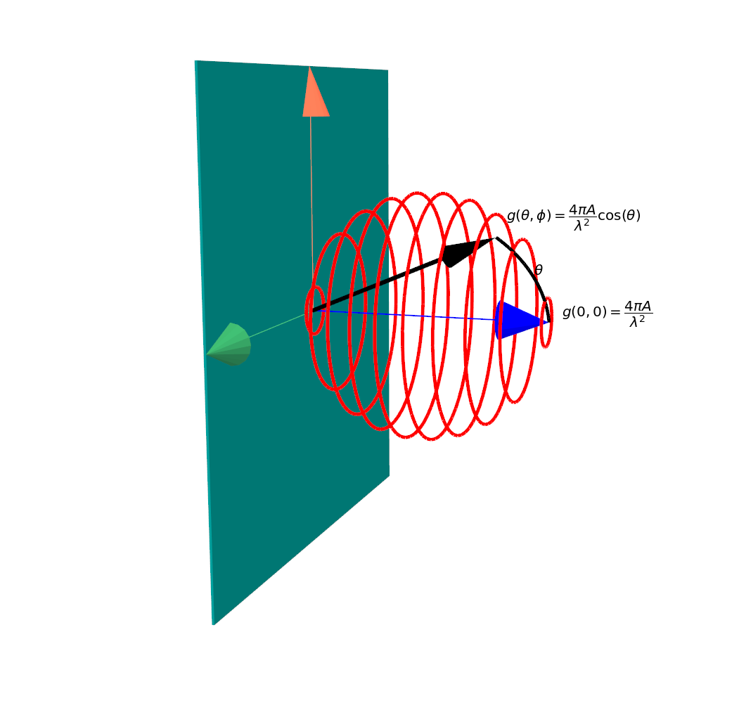Figure 1: Ideal Array Element Pattern for an array element.

What this means for beamforming, is that for a planar antenna array there is a fundamental limit on how much gain can be achieved at any angle. This can be addressed with different approaches in antenna design, but fundamentally these are based upon extending the array from a planar surface to a more 3D structure.

$g_{max}(\theta,\phi)=\dfrac{4\pi A}{\lambda^{2}}\cos(\theta)$

While this is a useful result for predicting the performance in isolation of a planar antenna array, it does not function as a useful figure of merit for comparing different antenna array designs, or different beamforming methods. This is where the concept of steering efficiency and steering efficiency product come into play.

Steering Efficiency and Steering Efficiency Product

In order to provide a useful assesment of the performance of an antenna array and allow comparison with other antenna array designs, the figure must include the relationship between the achieved gain and the maximum achievable gain, and the effects of scan loss on the antenna array performance.

The concept of steering efficiency $\eta_{s}$ was proposed by Marin and Hesselbarth in Figure of Merit for Beam-Steering Antennas [2]. This metric relates the fraction of the farfield which can be beamformed to with a scan loss of less than 3dB from the antenna array maximum directivity (Field of View in steradians).

$\eta_{s}=\dfrac{FOV}{4\pi}$

Thus an antenna array which can beamform in any direction without scan loss would have a steering efficiency of 1, while an antenna array which could only beamform in a small region around boresight would have a low steering efficiency. A visual example of this on the ideal antenna element pattern from Figure 1 is shown in Figure 2.

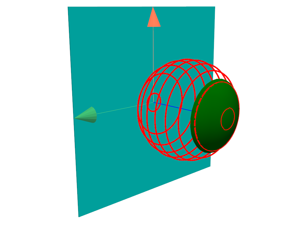Figure 2: Field of View (Green) for an antenna array

While steering efficiency is a useful metric in it’s own right, it does not account for the overall gain of the antenna array. This is where the steering efficiency product $\eta_{sep}$ comes into play. This metric combines the steering efficiency with the achieved gain of the antenna array at boresight as a fraction of the maximum possible gain (aperture efficiency $\eta_{ap}$), allowing a more comprehensive comparison of different antenna array designs and beamforming methods. Strictly $\eta_{ap}$ is defined as the ratio of the effective aperture of an antenna array to the physical aperture, and for realistic antenna arrays is always less than 1. Some example antenna arrays and horn antennas considered in [2] range in $\eta_{ap}$ from 0.18 to 0.64.

$\eta_{sep}=\eta_{ap}\dfrac{FOV}{4\pi}$

This can be demonstrated using the LyceanEM Array Beamforming example for a 10GHz conformal antenna array mounted on a UAV, as shown in Figure 2. The achieved gain at each command angle can be calculated using LyceanEM and Wavefront Beamforming, and the steering efficiency calculated.

This antenna array provides a steering efficiency of 3%. As LyceanEM does not include mutual coupling and other losses, the aperture efficiency is 100%, leading to a steering efficiency product of 3%. This can be observed by comparison to Figure 3 which shows the maximum directivity envelope for the antenna, and the effects of the sharply curving array and the blockages provided by the UAV itself on the achievable directivity.

Figure 3: Achieved Gain for a 10GHz Conformal Antenna Array mounted on a UAV.

While this does give a useful overview of the antenna array performance, it is not always very intuitive in terms of how the antenna array pattern changes with command angle. This is where an animation can be useful to give an understanding of the dynamics involved. A scan from $-90^{o}$ to $90^{o}$ in azimuth at $-15^{o}$ in elevation is shown in Figure 4. This animation was created using PyVista, and shows the achieved gain at each command angle, along with the UAV structure and antenna array geometry.

Figure 4: Animated Achieved Gain for a 10GHz Conformal Antenna Array mounted on a UAV, scanning from -90 to 90 in Azimuth

[1] P. Hannan, “The element-gain paradox for a phased-array antenna,” in IEEE Transactions on Antennas and Propagation, vol. 12, no. 4, pp. 423-433, July 1964, doi: 10.1109/TAP.1964.1138237 [2]: J. G. Marin and J. Hesselbarth, “Figure of Merit for Beam-Steering Antennas,” 2019 12th German Microwave Conference (GeMiC), Stuttgart, Germany, 2019, pp. 44-47, doi: 10.23919/GEMIC.2019.8698122